Examples

Prerequisites

We use the segmentation labels for OpenKnee(s) model 003 for these examples. You can download the segmentation labels in NIfTI format from the OpenKnee(s) datashare. The link should take you directly to OKS_models/oks003/segmentation after logging in.

To download just the segmentation labels, right-click on the segmentation folder and select Download.
SimTK will send a link to your registered email once the download is ready. You will need to follow this link to complete the download.
Create a directory in the seg2mesh root directory called dat and extract the downloaded ZIP file to this directory.
Optionally, remove the following files from the dat/oks003/segmentation directory as we will not be using them:
- oks003_FMR-L_AGS.nii
- oks003_FMR-M_AGS.nii
- oks003_FMR-P_AGS.nii
- oks003_PTR-L_AGS.nii
- oks003_PTR-M_AGS.nii
- oks003_PTR-S_AGS.nii
- oks003_TBR-L_AGS.nii
- oks003_TBR-M_AGS.nii
- oks003_TBR-P_AGS.nii

You should now have a file structure in seg2mesh/dat that looks like this:

└── oks003
    └── segmentation
        ├── oks003_ACL_AGS.nii
        ├── oks003_FBB_AGS.nii
        ├── oks003_FMB_AGS.nii
        ├── oks003_FMC_AGS_03.nii
        ├── oks003_LCL_AGS.nii
        ├── oks003_MCL_AGS_02.nii
        ├── oks003_MNS-L_AGS_02.nii
        ├── oks003_MNS-M_AGS_02.nii
        ├── oks003_PCL_AGS.nii
        ├── oks003_PTB_AGS.nii
        ├── oks003_PTC_AGS.nii
        ├── oks003_PTL_AGS.nii
        ├── oks003_QAT_AGS.nii
        ├── oks003_TBB_AGS.nii
        ├── oks003_TBC-L_AGS.nii
        └── oks003_TBC-M_AGS.nii

Congratulations! You are ready to run the examples.

Segmentation Label Volume Processing Pipeline

seg2mesh provides a pre-defined pipeline for processing segmentation label volumes. This is configured with a seg2mesh.config.SegmentationPipeline object. This object can be defined in code or read from a JSON file.

Example: Segmentation labels as unique files

Example JSON configuration for the volume processing pipeline using unique label files

{
  "source_files": [
    "../dat/oks003/segmentation/oks003_FBB_AGS.nii",
    "../dat/oks003/segmentation/oks003_FMB_AGS.nii",
    "../dat/oks003/segmentation/oks003_TBB_AGS.nii",
    "../dat/oks003/segmentation/oks003_PTB_AGS.nii",
    "../dat/oks003/segmentation/oks003_ACL_AGS.nii",
    "../dat/oks003/segmentation/oks003_LCL_AGS.nii",
    "../dat/oks003/segmentation/oks003_MCL_AGS_02.nii",
    "../dat/oks003/segmentation/oks003_PCL_AGS.nii",
    "../dat/oks003/segmentation/oks003_PTL_AGS.nii",
    "../dat/oks003/segmentation/oks003_QAT_AGS.nii",
    "../dat/oks003/segmentation/oks003_MNS-L_AGS_02.nii",
    "../dat/oks003/segmentation/oks003_MNS-M_AGS_02.nii",
    "../dat/oks003/segmentation/oks003_TBC-L_AGS.nii",
    "../dat/oks003/segmentation/oks003_TBC-M_AGS.nii",
    "../dat/oks003/segmentation/oks003_FMC_AGS_03.nii",
    "../dat/oks003/segmentation/oks003_PTC_AGS.nii"
  ],
  "output_path": "../dat/examples/openknee",
  "target_voxel_size": [0.25, 0.25, 0.25],
  "processing_options": {
    "close": true,
    "closing_radius": [4, 4, 4],
    "open_list": [
      "oks003_LCL_AGS",
      "oks003_MNS-L_AGS_02",
      "oks003_MNS-M_AGS_02"
    ],
    "opening_radius": [1, 1, 1],
    "spur_removal_length": 10,
    "make_contiguous": [
      ["oks003_FMC_AGS_03", "oks003_FMB_AGS"],
      ["oks003_TBC-L_AGS", "oks003_TBB_AGS"],
      ["oks003_TBC-M_AGS", "oks003_TBB_AGS"],
      ["oks003_PTC_AGS", "oks003_PTB_AGS"]
    ]
  }
}

To execute the pipeline as a script, from the examples directory, run:

uv run python -m seg2mesh.vol_pipeline process_oks_vol.json

Output files will be written to ../dat/examples/openknee as specified by the output_path attribute.

Additional command-line arguments for log_level and log_file can be specified. See help for seg2mesh.vol_pipeline by running:

uv run python -m seg2mesh.vol_pipeline --help

Note

The order of source_files matters. Later entries take precedence over earlier ones, if there is overclosure. We order the files as bones, then ligaments, then menisci, then cartilage. This ensures the thin cartilage structures take precedence, since changes in thickness will have very strong structural effects.

We can visualize the unprocessed.seg.nrrd and processed.seg.nrrd label images in supporting viewers. The following images and videos were generated using ParaView. Figure 1 is a slice through animation of the unprocessed and processed labels overlaid on the MRI (not provided in the prerequisite download). Generally, there are only subtle changes between labels, which is desirable. We really just want to reduce spurious (high frequency) features that will impact mesh creation later.

Figure 1: Slice through animation of the unprocessed and processed labels overlaid on the MRI.

Zooming in on a single slice, we can see the effects of make_contiguous in Figure 2.

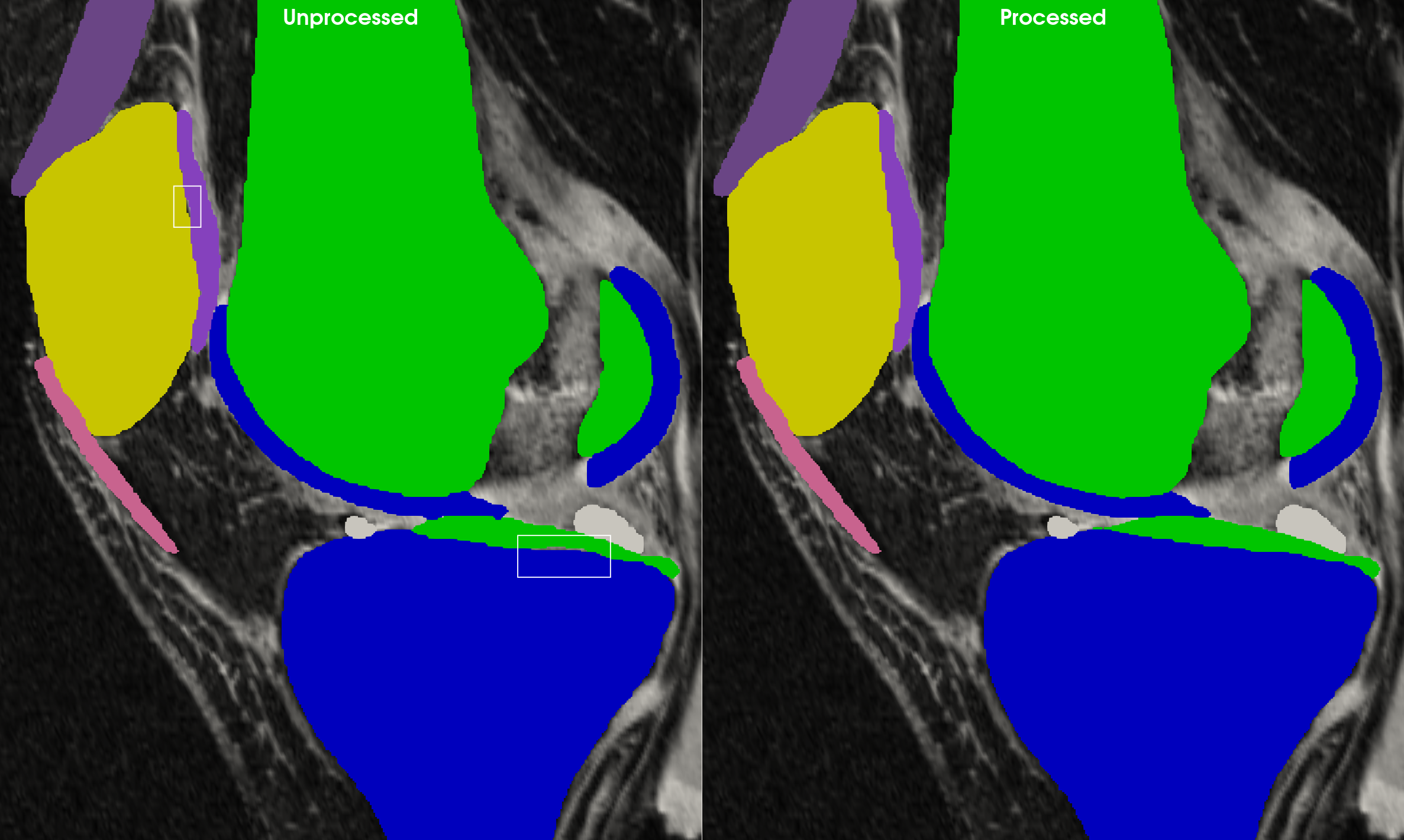
_images/overlay_contiguous_repair.png — Figure 2: A slightly zoomed single slice comparison of the unprocessed and processed labels. Notice the effects of make_contiguous on the cartilage regions outlined in white boxes. Click for a full-size version.

Example: Segmentation labels in a single file

The previous example demonstrated how to process files where each label was a separate image. It also built the Lookup Table (LUT) mapping each label “Short Name” to its integer value using the source_files list. The “Short Name” were automatically defined as each source_file stem (i.e., the filename without extension). When multiple labels are present in a single file, we do not have this option. Therefore, it is recommended to supply the lut attribute in the config. Notice the single source_file was generated by the previous example, so we already know the order of the integer labels. We also took the opportunity to shorten the names further. Notice how these shorter names are used in the open_list and make_contiguous attributes.

Note

If lut is not specified and there is a single item in source_files, the LUT will be automatically generated with keys defined as the str(label) where label is the integer values found in the image.

Example JSON configuration for volume processing pipeline using a single file containing multiple labels

{
  "source_files": ["../dat/examples/openknee/unprocessed.seg.nrrd"],
  "output_path": "../dat/examples/openknee_multilabel",
  "target_voxel_size": [0.25, 0.25, 0.25],
  "lut": {
    "FBB": 1,
    "FMB": 2,
    "TBB": 3,
    "PTB": 4,
    "ACL": 5,
    "LCL": 6,
    "MCL": 7,
    "PCL": 8,
    "PTL": 9,
    "QAT": 10,
    "MNS-L": 11,
    "MNS-M": 12,
    "TBC-L": 13,
    "TBC-M": 14,
    "FMC": 15,
    "PTC": 16
  },
  "processing_options": {
    "close": true,
    "closing_radius": [4, 4, 4],
    "open_list": ["LCL", "MNS-L", "MNS-M"],
    "opening_radius": [1, 1, 1],
    "spur_removal_length": 10,
    "make_contiguous": [
      ["FMC", "FMB"],
      ["TBC-L", "TBB"],
      ["TBC-M", "TBB"],
      ["PTC", "PTB"]
    ]
  }
}

Execute the pipeline as before with:

uv run python -m seg2mesh.vol_pipeline process_oks_multilabel_vol.json

Output files will be written to ../dat/examples/openknee_multilabel as specified by the output_path attribute.

Label Image to Mesh Pipeline

This pipeline first extracts each isocontour by its integer value. It then applies a sequence of optional smoothing, remeshing, and error calculation operations configured by the seg2mesh.config.SurfaceMeshPipeline class. Specifically, these are as follows:

Taubin smoothing: defined by taubin_smoothing_factor1 and taubin_iterations1 options. Turn off smoothing by setting taubin_iterations1 <= 0.
Remeshing: applied based on provided remesh_options. If None, no remeshing is performed. If remesh_options is seg2mesh.config.AcvdOptions, the Approximate Centroidal Voronoi Diagram (ACVD) algorithm is used to remesh the mesh, otherwise if it is seg2mesh.config.MmgOptions, the mmg3d remeshing library is used. Consult the class documentations for more details.
Taubin smoothing: defined by taubin_smoothing_factor2 and taubin_iterations2 options. Turn off smoothing by setting taubin_iterations2 <= 0.
Error metric calculation
- If calculate_distance_metrics is True, Hausdorff, Mean Symmetric Surface, and Root Mean Square Distance metrics are calculated.
- If calculate_classification_metrics is True, Dice Coefficient, Intersection over Union, and Accuracy metrics are calculated.
- Metrics are saved to disk as CSV and also appended to the final processed polydata as FieldData.

Note

If calculate_classification_metrics is True, one should also set voxel_edge to be similar to the voxel size of the label image. These metrics require a voxelization or the mesh, and it should be of similar or equal resolution as the original label volumes.

Example: Label image to mesh with uniform (ACVD) remeshing

For this first mesh extraction and processing example, we use the ACVD remeshing algorithm to create a mesh of nearly uniform edge length. After extracting the isocontours we first apply Taubin smoothing, then we remesh to a 0.75mm edge length using ACVD, then apply another soft Taubin smoothing operation. The JSON configuration for this example is shown below.

Example JSON configuration for extracting isocontour from a label intensity image and processing the resulting mesh.

{
  "label_file": "../dat/examples/openknee/processed.seg.nrrd",
  "lut_file": "../dat/examples/openknee/processed.seg.json",
  "output_path": "../dat/examples/openknee_acvd",
  "calculate_distance_metrics": true,
  "calculate_classification_metrics": true,
  "voxel_edge": 0.25,
  "taubin_smoothing_factor1": 0.8,
  "taubin_iterations1": 60,
  "taubin_smoothing_factor2": 0.2,
  "taubin_iterations2": 40,
  "remesh_options": { "edge_length": 0.75 },
  "output_formats": ["vtp", "stl"]
}

Execute the pipeline with:

uv run python -m seg2mesh.smesh_pipeline smesh_oks_acvd.json

We visualize the resulting meshes using the configured pipeline in Figure 3 and 4.

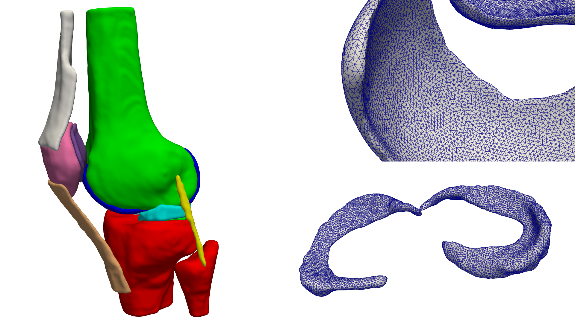
_images/acvd_mesh.png — Figure 3: The triangular meshes generated by the pipeline for the specified configuration. Zoomed in views of the femoral cartilage (top-right) and menisci (bottom-right) with mesh edges visible illustrate the uniform remeshing with ACVD.

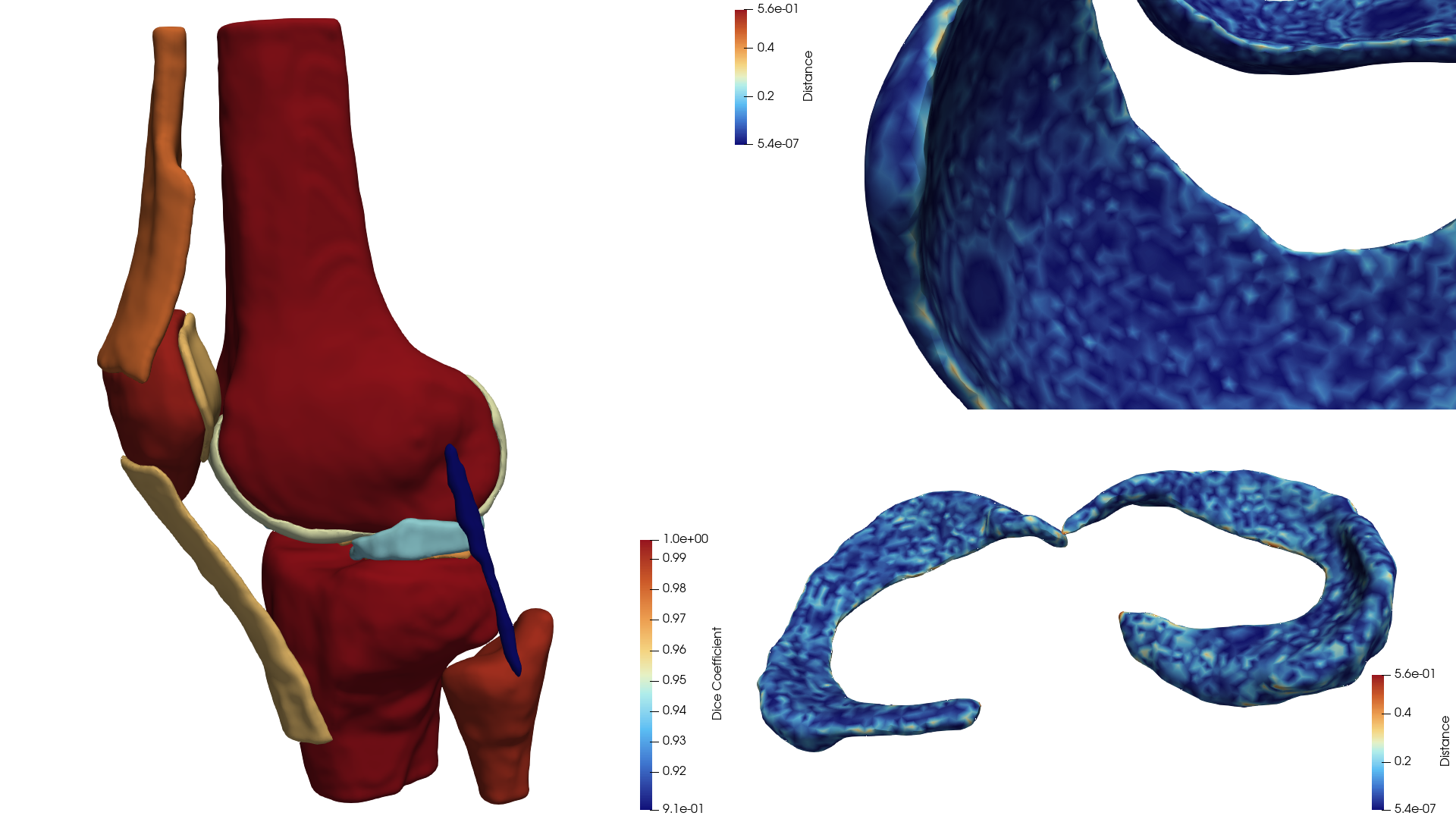
_images/acvd_error_metrics.png — Figure 3: Error metrics are stored when saved in VTP format. Aggregate measures like Dice Coefficient (left) are stored as FieldData. Per-vertex data like Distance (shortest distance from processed to unprocessed mesh) can be visualized as shown for the femoral cartilage (top-right) and menisci (bottom-right). Note the Distances are highest in areas of high curvature, like the thin cartilage edge, largely due to the use of uniform remeshing.

Example: Label image to mesh with adaptive (mmg3d) remeshing

For this mesh extraction and processing example, we instead use the MMG3D remeshing algorithm to create a mesh that is adapted to the local curvature of the initial mesh. This is controlled by the defining remesh_options as a seg2mesh.config.MmgOptions object. We clamp the curvature determined local edge length to hmin <= x <= hmax. After extracting the isocontours we first apply Taubin smoothing, then we adaptively remesh, then apply another soft Taubin smoothing operation. The JSON configuration for this example is shown below.

Example JSON configuration for extracting isocontour from a label intensity image and processing the resulting mesh.

{
  "label_file": "../dat/examples/openknee/processed.seg.nrrd",
  "lut_file": "../dat/examples/openknee/processed.seg.json",
  "output_path": "../dat/examples/openknee_mmg",
  "calculate_distance_metrics": true,
  "calculate_classification_metrics": true,
  "voxel_edge": 0.25,
  "taubin_smoothing_factor1": 0.8,
  "taubin_iterations1": 60,
  "taubin_smoothing_factor2": 0.2,
  "taubin_iterations2": 40,
  "remesh_options": {
    "hmin": 0.2,
    "hmax": 1.0,
    "hgrad": 1.5,
    "divisions_per_circle": 8.0
  },
  "output_formats": ["vtp", "stl"]
}

Execute the pipeline with:

uv run python -m seg2mesh.smesh_pipeline smesh_oks_mmg.json

We visualize the resulting meshes using the configured pipeline in Figure 5 and 6.

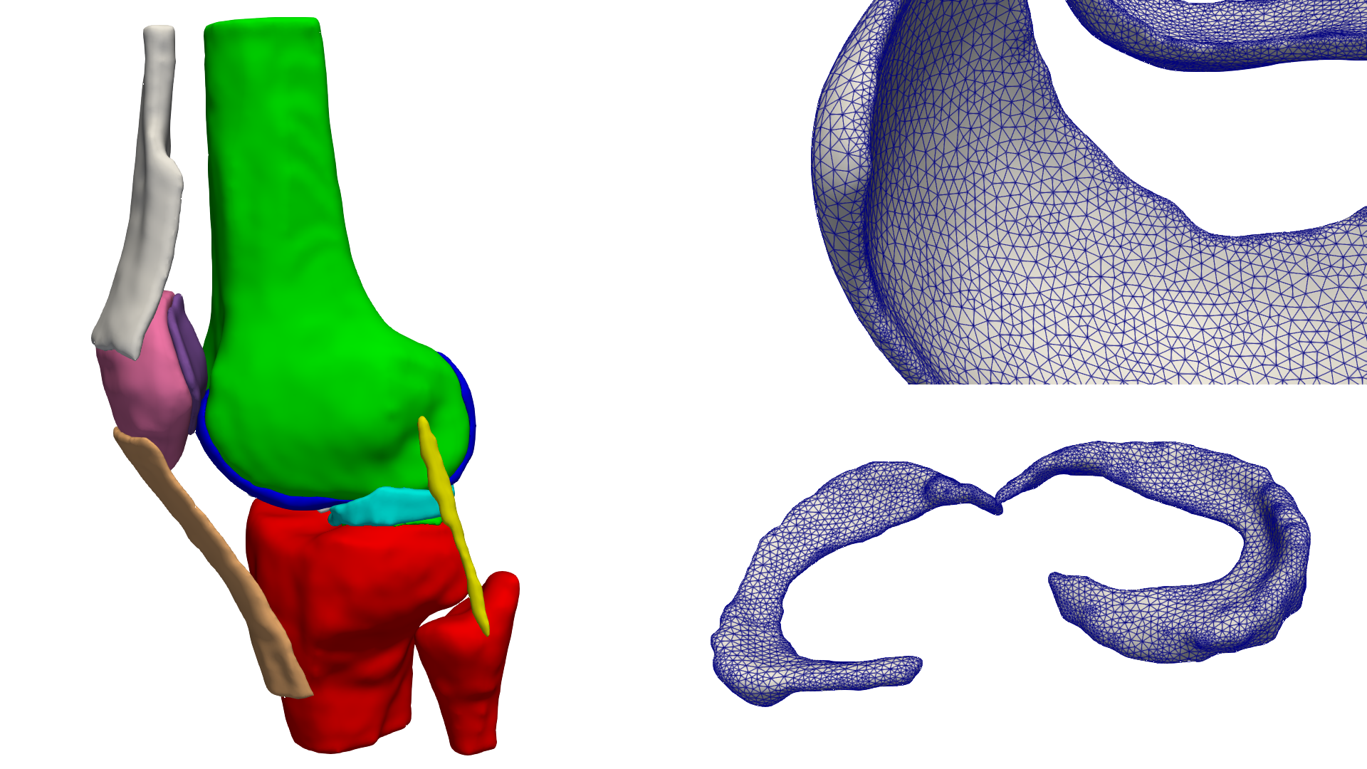
_images/mmg_mesh.png — Figure 5: The triangular meshes generated by the pipeline for the specified configuration. Zoomed in views of the femoral cartilage (top-right) and menisci (bottom-right) with mesh edges visible illustrate the adaptive remeshing with MMG3D.

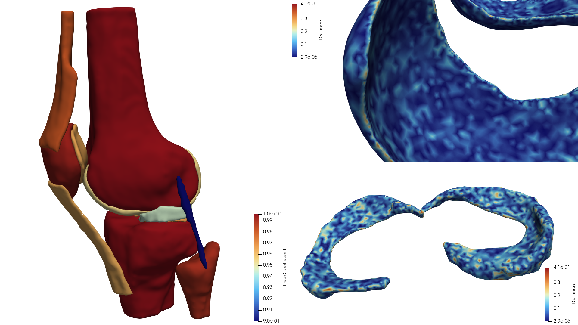
_images/mmg_error_metrics.png — Figure 6: Error metrics are stored when saved in VTP format. Aggregate measures like Dice Coefficient (left) are stored as FieldData. Per-vertex data like Distance (shortest distance from processed to unprocessed mesh) can be visualized as shown for the femoral cartilage (top-right) and menisci (bottom-right). Distances are still highest in areas of high curvature, but due to using adaptive remeshing, these are less than in the ACVD example.